Grid Creation and Grid-Based Descriptor Calculation
Another aspect of molli is it’s ability to create grids, as a lot of the Denmark lab workflows operate with grid-based descriptors.
Note: Pyvista is not natively installed within Molli, but this version can be added through conda using the line: pip install pyvista==0.43.10 or conda install pyvista=0.43.10
Grid Creation
[1]:
# Import the necessary packages
import molli as ml
import pyvista as pv

#This is currently being run on a virtual server and needs a separate server for display via pyvista
pv.start_xvfb()
[2]:
# Creates a rectangular grid as a canvas
g = ml.descriptor.rectangular_grid([-1,-1,0], [1,1,0], spacing=0.5)
print(g.shape)
g
(25, 3)
[2]:
array([[-1. , -1. ,  0. ],
       [-0.5, -1. ,  0. ],
       [ 0. , -1. ,  0. ],
       [ 0.5, -1. ,  0. ],
       [ 1. , -1. ,  0. ],
       [-1. , -0.5,  0. ],
       [-0.5, -0.5,  0. ],
       [ 0. , -0.5,  0. ],
       [ 0.5, -0.5,  0. ],
       [ 1. , -0.5,  0. ],
       [-1. ,  0. ,  0. ],
       [-0.5,  0. ,  0. ],
       [ 0. ,  0. ,  0. ],
       [ 0.5,  0. ,  0. ],
       [ 1. ,  0. ,  0. ],
       [-1. ,  0.5,  0. ],
       [-0.5,  0.5,  0. ],
       [ 0. ,  0.5,  0. ],
       [ 0.5,  0.5,  0. ],
       [ 1. ,  0.5,  0. ],
       [-1. ,  1. ,  0. ],
       [-0.5,  1. ,  0. ],
       [ 0. ,  1. ,  0. ],
       [ 0.5,  1. ,  0. ],
       [ 1. ,  1. ,  0. ]], dtype=float32)
[3]:
# Adds theme to Pyvista plot and allows for jupyter notebook integration
pv.set_plot_theme("dark")
plt = pv.Plotter(notebook=True)
# Creates a point cloud from the grid generated by molli and adds it to the plot
points = pv.PointSet(g)
# Adds more features to the plot and displays it
plt.add_mesh(points, color="cyan", render_points_as_spheres=True, point_size=10)
plt.add_axes_at_origin()
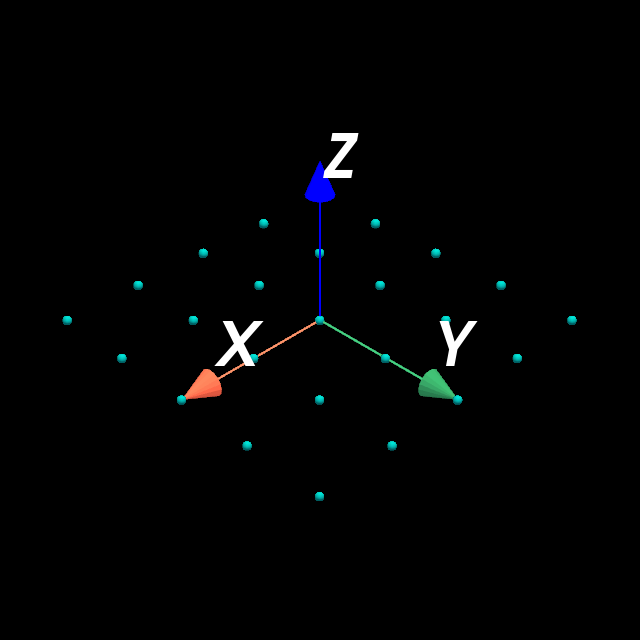
plt.show(jupyter_backend="panel", window_size=(640,640))
Grid-Based Conformer-Average (GBCA) Descriptor Calculation
The command-line interface within molli also allows rectangular grid calculation then subsequent descriptor calculation from an existing conformer library file. This can be parallelized, and will be returned as an hdf5 file.
Grid Calculation
An example command would look like
molli grid example.clib -o example_grid.hdf5 -s 1.0 -n 16 --prune
Note: The --prune option is necessary for the accelerated GBCA descriptor calculation, but unecessary for standard grid calculation
Other parameters available in the grid script are shown below
[4]:
!molli grid -h
usage: molli grid [-h] [-o <fpath>] [-n NPROCS] [-p 0.0] [-s 1.0]
                  [-b BATCHSIZE] [--prune [<max_dist>:<eps>]]
                  [--nearest [NEAREST]] [--overwrite] [--dtype DTYPE]
                  library

Read a molli library and calculate a grid

positional arguments:
  library               Conformer library file to perform the calculations on

options:
  -h, --help            show this help message and exit
  -o <fpath>, --output <fpath>
                        Destination for calculation results
  -n NPROCS, --nprocs NPROCS
                        Specifies the number of jobs for constructing a grid
  -p 0.0, --padding 0.0
                        The bounding box will be padded by this many angstroms
                        prior to grid construction
  -s 1.0, --spacing 1.0
                        Intervals at which the grid points will be placed
  -b BATCHSIZE, --batchsize BATCHSIZE
                        Number of molecules to be treated simulateneously
  --prune [<max_dist>:<eps>]
                        Obtain the pruning indices for each conformer ensemble
  --nearest [NEAREST]   Obtain nearest atom indices for conformer ensembles.
                        This is necessary for indicator field descriptors.
                        Accepts up to 1 parameter which corresponds to the
                        cutoff distance.
  --overwrite           Overwrite the existing grid file
  --dtype DTYPE         Specify the data format to be used for grid parameter
                        storage.
ASO/AEIF Calculation
The Average Steric Occupancy (ASO) descriptor was originally developed in the Denmark lab to capture the dynamic nature of sterics in a molecule. This measures whether an indiviudal conformer is occupying a grid point or not and assigns it a value of 0 if unoccupied and a value of 1 if occupied. This then averages the amount a grid-point was occupied over the number of conformers calculated, giving a value between 0 and 1. More information can be found at DOI:10.1126/science.aau5631
We have significantly accelerated this descriptor calculation such that it can operate on massive ConformerLibraries. This has also been made availble to parallelize for further acceleration. An example of an ASO calculation run through the command line is shown below
molli gbca aso example.clib -o example_aso.hdf5 -g example_grid.hdf5 -n 16
The Average Electronic Indicator Field (AEIF) descriptor has a very similar implementation as ASO, with the only difference being the grid-point is not assigned a 0 or 1 for occupancy, rather it is assigned the electronic charge of an atom.
Note: This requires the atomic charges for the ConformerEnsemble in each ConformerLibrary to be previously calculated and assigned.
Other parameters available in the gbca script are shown below
[5]:
!molli gbca -h
usage: molli gbca [-h] [-w] [-n 128] [-b 128] [-g <grid.hdf5>]
                  [-o <lib_aso.hdf5>] [--dtype DTYPE] [--overwrite]
                  {aso,aeif} CLIB_FILE

This module can be used for standalone computation of descriptors

positional arguments:
  {aso,aeif}            This selects the specific descriptor to compute.
  CLIB_FILE             Conformer library to perform the calculation on

options:
  -h, --help            show this help message and exit
  -w, --weighted        Apply the weights specified in the conformer files
  -n 128, --nprocs 128  Selects number of processors for python
                        multiprocessing application. If the program is
                        launched via MPI backend, this parameter is ignored.
  -b 128, --batchsize 128
                        Number of conformer ensembles to be processed in one
                        batch.
  -g <grid.hdf5>, --grid <grid.hdf5>
                        File that contains the information about the
                        gridpoints.
  -o <lib_aso.hdf5>, --output <lib_aso.hdf5>
                        File that contains the information about the
                        gridpoints.
  --dtype DTYPE         Specify the data format to be used for grid parameter
                        storage.
  --overwrite           Overwrite the existing descriptor file